LOW-RISK IOT DESIGN: How to Manage IoT Design Risks from Planning to Manufacture | Voler Systems
Overview

Data acquisition is the sampling of continuous real-world information to generate data that can be manipulated by a device, such as a computer. Acquired data can be displayed, analyzed, and stored. A PC or other device can be used to collect real-world information such as voltage, current, temperature, pressure, sound, chemical sensing, heart rate, and thousands of other parameters. The components of data acquisition systems include appropriate sensors, filters, signal conditioning, data acquisition devices, and application software. Ultimately data analysis can only be as good as the input data, so acquisition is responsible for providing high-quality data.
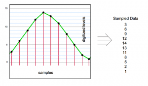
The most important concepts of data acquisition have to do with digitizing the data so a device with a processor can use it. For example, in the past you may have read data on a meter with a needle that moves back-and-forth. This is an analog representation of the data. The needle moves smoothly to any position. You may also read data on a digital meter that displays the data as numbers. This is a digital representation of the data, with changes in discrete steps where any step smaller than the resolution of the data acquisition device cannot be represented.
Not only is the data digitized in amplitude, but it is also digitized in time. Where the analog meter always shows the current input value, the digital meter does not. The digital meter is updated at a constant rate. It reads the value and displays it, perhaps ten times per second. Although the actual input value may change between readings, the meter does not change. The displayed value only changes when the next reading is made, every 100 milliseconds.
All modern data acquisition digitizes the data. The data is digitized in amplitude and time. It is easy to overlook the effect of the time digitizing, but it can be much more important than the amplitude digitizing. Consider an input signal that changes from 0 to 10 Volts in once second. A digital meter with three digits can resolve a change of 10 millivolts. If it updates only 10 times per second it will change one Volt at each sample. This is the equivalent of having only one digit of resolution (or 10% resolution), because the change from one sample to the next is a change of one digit in the most significant or left-most digit. When reading a digital meter this is usually not a problem. When collecting data for analysis this can be a big problem.
From the above discussion, it is clear that you need to determine the sample rate of a data acquisition system with care, but how do you choose? For slowly changing signals, like temperature, the only consideration is to provide a new reading so that the data is reasonably up-to-date. If the temperature is read only once per minute, it may not accurately display the temperature of an oven that is heating rapidly. A faster sample rate is necessary.
In some applications it is necessary to accurately represent an input waveform. An electrocardiogram, for example, must be reproduced with considerable precision because some of the important things a doctor looks for are small changes in the waveform. To accurately display such a waveform, you can look at the fastest rate-of-change in the signal, expressed in Volts per second.
In the example above of the digital meter, the signal changed at one Volt per second (which is much slower than an electrocardiogram). To detect a change as small as 1% of the 10 Volt signal it is necessary to sample 100 times per second. To detect a change of 0.1% of the 10 Volt signal it is necessary to sample 1000 times per second. The electrocardiogram signal changes rapidly in a short time. The standard for electrocardiogram signals is to sample 500 times per second, even though the heart rate is about once per second.
In many applications the accurate representation of the waveform is not very important, but representing all frequency components of the signal is important. Without going into the math, the Nyquist theorem states that the sample rate must be at least twice the highest frequency in order to measure all the frequencies present.

Aliased Signal
In fact, if the sample rate is too slow, you not only don’t measure the highest frequency, but lower frequencies are created in the data that didn’t exist in the input signal! The diagram below shows a high frequency “original signal” with a sample rate a little below the frequency of the original signal (shown as red lines). When the red lines are connected to show the signal they represent (green lines), a much lower frequency emerges, the “signal created by aliasing”.
In a vibration signal, the frequency of vibration is almost always very important. If the sample rate is so slow that the data shows frequencies that didn’t really exist, the data is completely wrong. Instead of calculating the fastest rate of change in the signal, you determine the highest frequency component that will cause a change. Thus, for some signals, especially vibration, the avoidance of aliasing is the main factor you need to consider for sample rate.
An electronic filter can be used to separate wanted signal from noise. Since there is the possibility of frequencies higher than half the sample rate (often due to noise), a filter is almost always used in vibration measurement applications. If the filter is ideal (which it never is) the sample rate must be at least twice the cut-off frequency of the filter, the frequency above which no signal can pass through. Since real filters allow some signals to pass through above the cut-off frequency, the sample rate must be greater than twice the cut-off frequency. It is complicated to figure the necessary frequency, but it is often 4 to 10 times the cut-off frequency, depending upon the filter characteristics.
Filters are characterized by the number of “poles” they have. A pole is a mathematical characteristic that comes from the complexity of the filter. A more complex filter has more poles and more closely approaches an ideal filter.
You can see from the diagram that a simple one-pole filter is not very good at blocking frequencies above the cut-off frequency. A signal that is time times the cut-off frequency is only attenuated 10 times. This may not be enough to prevent aliasing.

Ideal and practical filters
Data acquisition software can be simple and straight-forward when sample rates are slow. Polled (or asynchronous) acquisition can be used, in which the application determines when to sample data from the data acquisition device, one sample at-a-time. This does not work with high-speed data, because of the overhead involved in acquiring each sample.
Interrupt driven (or synchronous or buffered) acquisition acquires data in blocks, acquiring many samples at once with virtually the same overhead as for one sample in polled acquisition. Interrupt acquisition can give sample rates 10 to 1000 times faster than polled. Also, the time between samples is much more precise. Along with these benefits there is more complexity, whether writing data acquisition software or simply configuring it. The following explains how to configure a data acquisition application that does interrupt driven acquisition. Acquired data can be analog inputs, digital inputs, or counter/timer inputs. Outputs work in a similar fashion.
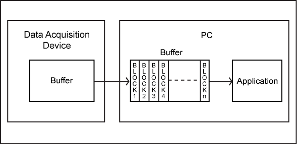
To capture data rapidly and at precisely timed intervals, the low-level data acquisition driver does the work, putting one sample after another into a portion of the memory referred to as a buffer. The application takes the data out of the buffer for analysis, not one sample at-a-time, but in blocks of many samples. In this example there is a device connected to a personal computer (PC).

The low-level data acquisition driver talks directly to the hardware, manipulating the registers of a data acquisition device. The driver is written to be small and fast so it can rapidly put data into the buffer.
In the application you specify a block size and sample rate. The low-level driver fills the buffer at the specified sample rate. The application must wait until enough data is acquired to fill one block. Then it can process all the data from the entire block. After that it must wait until the next block of data is full before it can process any more data.
In interrupt driven data acquisition there are two independent processes, the data acquisition driver reading data and putting it into the buffer, and the application taking data out of the buffer and processing it. Each process has its speed limitation.
Typically, the driver can put data into the buffer faster than the application can process it. If the data acquisition device is running at its maximum rate the buffer may eventually fill because the application does not process the blocks of data fast enough.
When the buffer fills with unprocessed data there are two options. The application can stop processing and display a warning message, or data in the buffer can be overwritten. It is rarely acceptable to overwrite data, so most data acquisition applications stop when the buffer fills.
What the operator of the application sees is that the application runs for a while then stops and says the sample rate is too fast. If the buffer is very large it could take many minutes before the buffer fills and the application stops. To give the operator an indication that the buffer is filling, it is desirable to have an indicator showing the status of the buffer. As the buffer fills with unprocessed data the status moves from 0% to 100% full.
Many data acquisition devices have their own data buffers, separate from the buffer in the PC memory discussed above. The data acquisition driver can transfer data from the buffer on the data acquisition device to the buffer in PC memory in blocks. This speeds up the data acquisition into the PC buffer.

Having a buffer on the data acquisition device increases the speed for the same reason that the buffer in the PC memory increases the speed. The overhead of processing one sample in the driver is the same for processing many samples. This is especially critical in complex operating systems such as Windows or Linux.
When the buffer is in the device the same issues arise as with a buffer in PC memory. The data is processed in blocks, and the buffer can overflow.
Typically, the data acquisition driver is activated by interrupts generated by the data acquisition device. If the device has no buffer the PC must be interrupted each time a sample is available. The interrupt causes the processor in the PC to stop what it is doing and execute the driver program. The driver must transfer the data from the data acquisition device to the PC memory buffer and return to allow the PC to resume what it was doing before another interrupt occurs. In Windows this can reliably run up to about 1000 samples per second. If another application is running or if the application does a lot of processing the speed may be limited to much less.
If the data acquisition device has a buffer, many samples may be transferred during each interrupt. With a buffer of just 1000 samples a maximum speed of 1,000,000 samples per second is possible (if the device can run that fast), or at slower speeds the application can perform complex processing, or another application can run simultaneously without losing data. In Windows other applications or drivers may run without your knowledge. Having a buffer on the data acquisition device is very valuable when you want to collect fast data at a constant rate.
When a small device collects data, the same issues apply. A device worn on your wrist may run an operating system such as Linux, and there may be a section of the device that collects data into a separate buffer. All of this can fit into a tiny device on your wrist.
As you can see, although interrupt data acquisition allows much faster sampling rates, there is an inherent delay between the reading of the data and the processing of it. The data appears on the screen or is logged to disk after the delay. In addition, there is a small delay due to the processing in the application. Most drivers and applications work together in such a way that the time reported for the data sample is the actual time that it was acquired, not when it was put into the buffer, and not when it was processed by the application.
The following table shows the time delay to fill a block of data and the time delay before the data appears on disk for an application that is logging data to disk. Not included is the delay due to the file buffer, which is set outside the application. This additional delay is not noticeable unless power is lost. Data still in the file buffer (or for that matter, the PC memory buffer) and not yet written to disk is lost during a power outage.
The table assumes there is a delay of 0.1 seconds for the application to process the data. Depending upon what the application is configured to do, this could be much larger, perhaps one second or more.
| Time delay after sampling an input | |||
| Sample Rate | Block Size | Buffer Delay | Delay to Disk |
| (Hz) | (Samples) | (Seconds) | (Seconds) |
| 10,000 | 10,000 | 1 | 1.1 |
| 10,000 | 1,000 | 0.1 | 1.2 |
| 1,000 | 10,000 | 10 | 10.1 |
| 1,000 | 1,000 | 1 | 1.1 |
| 1,000 | 100 | 0.1 | 0.2 |
| 100 | 10,000 | 100 | 100.1 |
| 100 | 1,000 | 10 | 10.1 |
| 100 | 100 | 1 | 1.1 |
For data acquisition devices with their own on-board buffer, the delay is the same as the chart above as long as the size of the buffer is less than the block size of the application. If the device buffer is set smaller than the block size in the application the application will have to wait for the device buffer to fill before it can process any data. Many data acquisition devices can transfer small amounts of data from the device buffer to the PC memory buffer to avoid this problem when sample rates are slow.
Be sure that the PC memory buffer is larger than the device buffer or the PC memory buffer could overflow, stopping data acquisition, even when the sample rate is quite slow.
When acquiring data from a data acquisition device there is normally a time delay between channels. Most data acquisition devices use a multiplexer to sample one input after the other in sequence. As a result, the channels are not read simultaneously.
With some drivers and data acquisition devices the time between channels is spaced evenly throughout the entire sampling interval to give the maximum settling time for the amplifier after switching between channels. With other drivers and data acquisition devices the time between channels is kept to a minimum by scanning through the channels at maximum speed then waiting for the next sample interval. Because the channels are nearly simultaneous this is sometimes called pseudosimultaneous acquisition.
When data is logged to a disk it is usually time stamped with the time of acquisition of the first channel. It appears that all the channels were sampled at the same time, which is not true. In fact, the data on the disk is sampled as shown in the following tables.
Sample Times, Sample Rate 100 Hz, 4 Channels, Time in ms
| Evenly Spaced Acquisition | ||||
| Sample | Channel 1 | Channel 2 | Channel 3 | Channel 4 |
| 1 | 0 ms | 2.5 ms | 5 ms | 7.5 ms |
| 2 | 10 ms | 12.5 ms | 15 ms | 17.5 ms |
| 3 | 20 ms | 22.5 ms | 25 ms | 27.5 ms |
| Pseudosimultaneous Acquisition | ||||
| Sample | Channel 1 | Channel 2 | Channel 3 | Channel 4 |
| 1 | 0 ms | 0.01 ms | 0.02 ms | 0.03 ms |
| 2 | 10 ms | 10.01 ms | 10.02 ms | 10.03 ms |
| 3 | 20 ms | 20.01 ms | 20.02 ms | 20.03 ms |
This table shows the time delay in the actual acquisition of the data. It does not include the delay due to filling the buffer and processing the data by the application that is described above. In this pseudosimultaneous acquisition example the time between channels is 10 us. The particular data acquisition device determines this. The time is normally determined by the maximum sample rate. A maximum rate of 100,000 samples per second yields a time between samples of 10 us.
There are devices that collect multiple channels simultaneously. This is called “simultaneous sample-and-hold” or SSH. These devices capture the analog value of all channels simultaneously, then they digitize the samples one-at-a-time. This eliminates the time skew between channels. In some applications, such as vibration measurement, the time skew is critical and affects the results of the data analysis, so SSH is very important to getting good data.
Continuous acquisition of data at rates over 100,000 samples per second can be achieved in Windows software. At these rates data can only be streamed to disk in binary format. If any processing of the data in the application is desired, if the acquisition device is limited in speed, or if data rates above this are desired it is necessary to capture data in a burst.
Data acquisition in bursts is always done synchronously so the sample rate is precise. The PC memory buffer is filled with a burst of data while the application is inactive and not using any processor resources. Once the buffer is full the application takes over and processes the data. The acquisition burst may be restarted manually, or in some software it can start again automatically. There is a gap between each burst while the application processes the data during which no data is captured.
You must specify ahead of time the number of samples to take in a burst. The maximum number of samples is limited by the amount of memory in the PC. In continuous mode the number of samples is essentially unlimited or is limited to the amount of disk space when logging data to disk.
Burst mode acquisition is even faster when the data acquisition device has its own buffer. The rate of acquisition is limited only by the speed of the device and the size of its buffer. Usually, PCs have more memory than data acquisition devices, so more samples can be taken in burst mode into the PC memory, but the speed is slower.
Many data acquisition software applications offer a compromise between continuous acquisition and burst acquisition. Streaming to disk moves data very efficiently from the data acquisition device to a disk drive. It is much faster than continuous acquisition because no other processing or display is done. It is slower than burst acquisition, but the amount of data that can be captured is limited by the space available on the disk, rather than in memory.
All the inputs discussed up to now have been analog inputs. There are applications where fast switching digital signals need to be counted or the frequency needs to be measured. This is often most conveniently done with a hardware counter/timer. A hardware counter/timer can count 10 million to billions of digital pulses per second.
The application software reads the number of pulses counted. This happens at the sample rate specified for inputs. When doing synchronous data acquisition, the pulse count is read into the buffer by the driver, just as with analog inputs. The application software reads data out of the buffer in blocks, just as with analog inputs. The pulse count may be read slowly, for example at 100 samples per second, even though the pulses are counted at a fast rate, for example 1,000,000 pulses per second. In this example each time the pulse count is read (each sample) there will be about 10,000 pulses (0.01 second at 1,000,000 samples per second).
If you want to measure the total number of pulses, you should set up the application software to calculate the total number of pulses from all the samples, adding the number from each sample. If you want to measure the frequency, the application software must divide the number of pulses during each sample by the length of the sample interval.
You must pay attention to how precisely you want to resolve the frequency by choosing the sample rate compared to the pulse rate. For example, if the sample rate is 1,000 samples per second and the pulses being measured are 10,000 Hz, there are 10 pulses in each sample. The frequency can only be resolved to 10% of 10,000 Hz (resolution of 1,000 Hz) because changes in frequency are discrete. There are either 9 or 10 or 11 pulses in a sample, yielding frequencies of 9,090 Hz, 10,000 Hz, or 11,111 Hz.
There are two ways to resolve the frequency to a finer precision: 1) reduce the sample rate so more pulses are measured in each sample, or 2) average the resulting frequency. Either way is equivalent. Reducing the sample frequency to 100 Hz or averaging 10 samples resolves the frequency to 1%, because there are 100 pulses in the sample (case 1) or in the average (case 2). It is more common to use the second method, because other factors may determine the sample frequency, such as the rate at which analog inputs need to be sampled.
Noise is unwanted interference that affects the signal and may distort the information. Noise comes from a variety of sources. Some comes from inside a circuit or device, and some comes from outside. Noise gets into a circuit from outside through two fundamentally different ways:
Radiated – like an antenna
Conducted – on wires
Radiated noise travels through the air as radio waves. To couple into a circuit or pass through an enclosure efficiently, the dimensions of the circuit or the hole in the enclosure must be close to one quarter of the wavelength of the noise. Here are wavelengths for various frequencies (in a vacuum):
1 KHz – 190 miles
1 MHz – 1000 feet
1 GHz – 1 foot
You can see that for most circuits the radiated noise is mainly a problem above 100 MHz, although AM radio stations (near 1 MHz) can induce significant noise in a circuit.
Metal enclosures and shielded cables are effective at reducing radiated noise. Keep in mind that an opening, even a slot, that is at ¼ wavelength is very efficient at letting signals through an enclosure. At frequencies of 1 GHz and above these slots can be hard to avoid.
Conducted noise gets into a circuit on wires. These can be the signal wires picking up the measured signal, or they can be the power supply wires. Battery operated devices avoid noise from the power supply wires. In addition to high frequency noise there is power line frequency noise, which is usually 50Hz or 60Hz. Two paths into your system are directly from the power line in power supplies and from coupling between signal wires and the power lines that run throughout most buildings.
The conducted noise is reduced by shielding or filtering. Shielding keeps the noise out, and filtering reduces it when all of it can’t be kept out of a circuit. If the signal being measured changes slowly, like temperature, the filter can have a low cut-off frequency. This makes it relatively easy to measure microvolt level signals from thermocouples. Signals such as accelerometers are often measured at 10 KHz, so the filtering cannot reduce as much noise.
Reducing noise is a big topic, beyond the scope of this paper. Voler Systems engineers are experts at data acquisition and noise reduction.
Analysis can only be as good as the input data. Careful data acquisition is responsible for providing high-quality data. This whitepaper looked at example architecture’s impact on sampling rate. Some other topics covered are common types of noise and techniques that are effective ways to reduce unwanted signals.
Do you have a question about our services, pricing, samples, resources, or anything else?
